MatricesMatrix Arithmetic
Matrix Multiplication
We learned in the last chapter that matrices can represent linear transformations. However, there are many other things that matrices can represent! Also, matrices do not always have to be
Four friends are in a new city and they're looking for a restaurant to eat at together. What are some features they might look for in a restaurant?
- Outdoor seating
- Vegetarian food
- Low price
- Spicy food
- Kid's menu
- Good wine selection
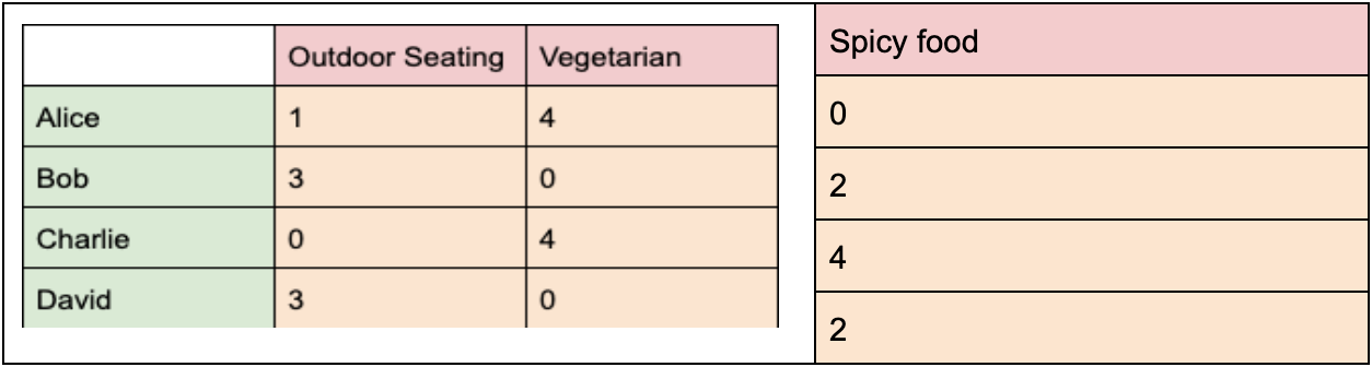
Each friend has preferences for how important these things are, which we can quantify with a value 0 (not important) to 4 (very important). If we create a table with friends on the left-most column and restaurant features across the top row, we can fill in the cells of the table with each friend's preference for that feature.
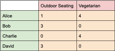
What we have built here is a 4 by 2 matrix. We have four rows to represent the four
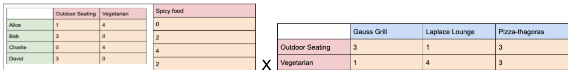
The friends have found three restaurants within walking distance, and they have pulled up the websites for each. Lucky for them, each restaurants' website has listed the quality of the features that the friends have quantified: availability of outdoor seating, and vegetarian options.
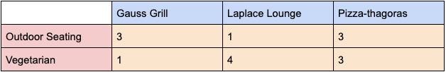
This is a 2 by 3 matrix. There are two rows to represent the two
Begin side-by-side column display.
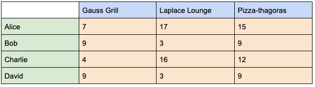
What we would like to do is somehow synthesize these two tables of information so we can get a sense of how much each person might like each restaurant. We can use a procedure called
How should we fill out this table? The value of each cell should represent how much each person might like each restaurant.
For example, the first cell will represent how much Alice might like
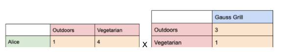
Alice has a preference of 1 for Outdoor Seating, and Gauss Grill has a value of 3 for Outdoor Seating, and we multiply these to get
Alice has a preference of 4 for Vegetarian food, but Gauss Grill only has a value of 1 for Vegetarian food, and we mutiply these to get
We sum together all the products to get
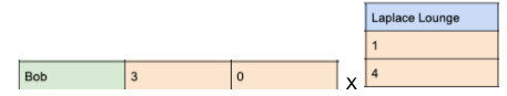
How much might Bob like Laplace Lounge?
When we finish our process, we get a matrix of 4 rows and 3 columns. This makes sense! We had 4 people and 3 restaurants, so we will end up with a row for each person and a column for each restaurant.
We can then sum the values in each column to figure out which restaurant is most popular (this is left as an exercise for the reader).
End side-by-side column display.
What we have just done is
Align these.
Formal definition of Matrix Multiplication
The formal defintion for matrix multiplication is as follows:
Given matrix
The value of the cell
where
Notice that, for this algorithm to work, the number of
For example, if in our restaurant example, each friend had a preference level for spicy food, our preference matrix would be
We are now attempting to multiply a
Could end section with a simple checkmark multiple choice, for which multiplications are possible.
Matrix Factorisation
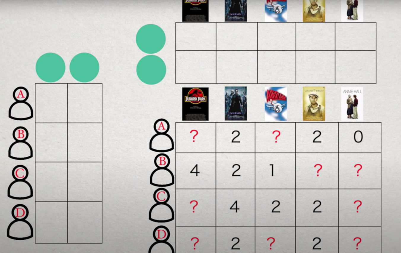
This type of matrix is used in all sorts of online recommender systems. Movies can be categorized by their genres like Comedy, Action, Romance, or Horror. Songs can be categorized into genres with ever-increasing specificity like Rock, Classical, Pop, Rap, Electro-Funk, Indie Folk, or Norwegian Black Metal. When you watch a movie on Netflix, or listen to a song on Spotify, there's likely a very large matrix somewhere, remembering your taste!
However, this process is slightly different from what we did above. The company running the streaming service doesn't know what its users' tastes are. It does know what movies they have watched, and whether they liked them or not. From this information they attempt to figure out each user's possible genre preferences using a process called matrix factorisation. Much like in
Multiplying Linear Transformations
We have now learned two different ways to think about matrix multiplication. In the first chapter we learned that multiplying a 2x2 matrix by a 2x1 vector, can be thought of as a linear transformation. And we just learned to the detailed rules for how to multiply matrices of any size, like a preference matrix. Let's go back to thinking about matrices as linear transformations.
Recall the 2x2 matrix representing the rotation of 90º about the origin. Let's call it
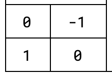
What if we multiply this matrix by the 2x2 matrix for rotation of 180º,
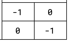
The resulting matrix is this:
This matrix is the linear transformation for a
That's right,
In this case, multiplying two rotation matrices give us a new rotation matrix with an angle equal to the sum of the first two angles. A more general way to say this is that when we multiplied two transformation matrices, the resulting transformation matrix has the effect applying BOTH of the original two matrices in succession.
This works for all rotation values:
R 90 R 90 R 80 R 180 R 180 R 360 I
What about other types of transformations?
Perhaps let them draw points (like a spaceship), and then the points are transformed by each transformation? {.fixme} Should be displayed horizontally, with their matrices across the bottom.
Matrix Addition
Matrices can also be added. Matrix addition does not happen very often, but it is very simple to learn.
We write matrix arithmetic just as you might expect:
- Two matrices can be added only if they have the same dimensions.
- The resulting matrix will be the same dimension as the matrices added.
- Each value in location (i,j) of the resulting matrix will be the sum of the values at (i,j) in the other two matrices.
Add these two matrices!
| 1 | 2 |
| 3 | 4 |
| 9 | 8 |
| 7 | 6 |
| | |
| | |
Great.
This code could be a lot simpler! And why is this not going below the tables?
Scalar Multiplication
Another operation we can perform with a matrix is scalar multiplication. A scalar is what we call a real number in matrix and vector arithmetic.
We write scalar multiplication as
Scalar multiplication is as simple as multiplying every cell in a matrix
| 3 | 1 |
| -4 | 0 |
| | |
| | |
Note that while it is possible to add two matrices, and to multiply a matrix by a scalar, the operation of adding a scalar to a matrix is not defined.
Properties of Matrix Arithmetic
Recall operators like addition and multiplication, and how it's useful to think about their properties. Commutative, distributive, and associative properties.
Associative
Is matrix multiplication
A good first question to ask is: will the dimensions of the matrices allow this?
If
We know we can perform this multiplication based on the dimensions, but will we get the same result? Recall from our section on multiplication that it can be thought of as successive linear transformations.
It turns out that as long as we keep the ordering of the matrices, we will get the same result. Whether we do BxC first or AxB first, it does not matter.
Matrix multiplication is associative.
Commutative
Is matrix multiplication
Recall that when we multiply two matrices, the number of columns of the first must match the number of rows of the second. This means that if we can multiply
What if both matrices are square matrices? We can then perform both
If we think of the matrices as transformations, we can imagine scenarios wherein applying two different transformations will be different depending on which direction you multiply them.
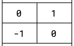
If we perform a 90º Rotation, and then a reflection across the x-axis, the final transformation will look like this:
However, if we reverse the order of the transformations, the final transformation will look like this.
There are many more examples of how matrix multiplication does not meet the commutative property, and we encourage you to experiment!
Distributive
Is matrix multiplication
Could demonstrate this by adding basis vectors and applying transformations to them. Or could somehow leave it as an exercise for the reader.