Introduction to ProbabilityIntroduction

In previous courses, we have seen how we can use science and mathematics to try to predict the future. For example, we can predict when a car will arrive at its destination if it is driving at a constant speed.

However, there are many examples in life where it is impossible to predict exactly what will happen. This could be because we don’t have all the information we need, because the decisions of other people might influence the result, or just because it is incredibly complicated.

Continue

Our language has many words we can use to describe the answer to these questions, without knowing exactly what will happen. Try to move each of these events to the best possible description:

You might have noticed that some of the descriptions were a bit “imprecise”. For example, if you roll a die just once, it is unlikely that it lands on a 6 – but you certainly wouldn’t be surprised if it does. WInning the lottery is unlikely too - but obviously, more unlikely than rolling that 6!

Unfortunately, our four word scale to describe the likelihood or chance of events occurring isn’t too useful.

One way to determine more accurately how likely a certain outcome is, is to look at how often it has happened in the past. For example, Imagine you’re playing a game of darts with your friend - and you want to numerically know how likely it is that your friend hits the bullseye. You could try to come up with some model to measure his skill, and learn how “good” he is - but a far easier method would be to listen to what his history says. In this case, your friend threw ${20} darts, ${5} of which landed in the center.

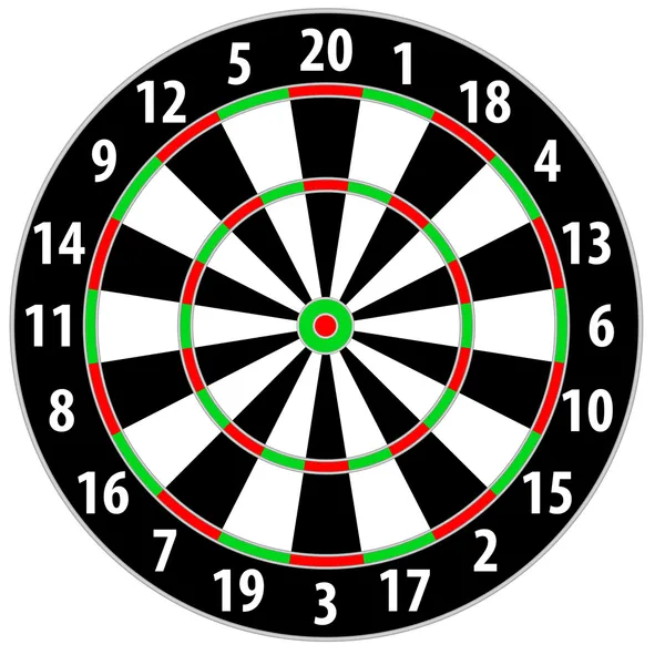
From this, you might deduce that the next throw has a 520=0.25 chance to also land in the center. We say that 0.25 is the probability of hitting the center.

For many centuries, mathematicians have struggled to deal with these uncertain situations – until the development of probability theory. In this course, we will explore what probability is, and give you some amazing new tools to be able to predict the future.

If you move the sliders above, you might notice that the probability is always between (if you never hit the center) and (if you always hit the center).

Probabilities always lie between 0 and 1. An event with a smaller probability (like 0.2) is always less likely than an event with a larger probability (like 0.8). If an outcome is impossible, we say it has probability 0. If it is certain, we say it has probability 1. If an event is equally likely to happen or not happen, its probability is exactly in the middle: .

We can represent probabilities using a number line from 0 to 1. Try to drag the following words and events onto the line, to show their approximate probability:

There are several different ways to represent probabilities, and we have already seen two of them. In the first example above, 5 out of 20 of the dart throws landed in the center.

We already know how to convert between fractions, decimals, and percentages, and we can do exactly the same for probabilities. Percentage literally means “Out of 100” - so 30% is the same thing as 30 times out of 100, or 30100!

Here are a few more predictions and events. Connect the ones that correspond to the same probability:

At this point, so start to suspect something. Maybe your friend is using a trick coin (or biased coin), where one side is weighted, and so the coin is more likely to land on it. But maybe you’ve also just been really unlucky! What do you think?

UnluckyTrick Coin

Probabilities can give us a sense of how likely a certain outcome is, but they don’t predict the future. Even if the weather forecast says there is only a 5% chance of rain, it might still happen. And our coin doesn’t “remember” the previous outcomes: every flip has the same probability of landing heads, which doesn’t depend on how many heads there were previously.

However, probabilities become much more useful if we can repeat the same experiment many times. For example, we could flip the same coin 100 times and compare how many heads and tails there are in total. Here are three different coins – can you work out which one of them is biased?

In the simulation above, when we used a fair coin (blue) - which has an equal probability of landing on heads and tails. As you can see, the graphs of the fair coins slowly approach 0.5 as you flip them more and more times. But the first tosses seem completely random, for both the fair and the biased coins.

Maybe you performed 10 tosses, and 8 coins landed on heads - you might think that the coin is biased immediately! However, it’s too soon to make that conclusion - If you reset the simulation, and keep tossing the coin just 10 times, you’ll see that the graph formed can be very jagged, and each repetition is different from the previous.

However, If you keep tossing the coin for another 100, or 1000 tosses: you’ll see that the ratio of Heads will always approach 0.5, out actual probability.

In probability theory, this phenomenon is known as the “Law of Large numbers” - The frequency of an event occurring in an experiment might not exactly match the actual probability of that event, but as the experiment is repeated many times, this frequency approaches the actual probability.

Whenever performing an experiment to find the probability of an event, it’s very important to perform it enough times - Else you might select the wrong coin to wager on!